Pandas is a an open source library providing tabular data structures and data analysis tools.In other words, if you can imagine the data in an Excel spreadsheet, then Pandas is the tool for the job.
Package Imports
This will be our first experience with importing a package.
Usually we import pandas with the alias pd.
We might also need numpy, Python’s main library for numerical computations.
import numpy as np
import pandas as pdSeries
A Series represents a one-dimensional array of data. It is similar to a dictionary consisting of an index and values, but has more functions.
names = ["Neckarwestheim", "Isar 2", "Emsland"]
values = [1269, 1365, 1290]
s = pd.Series(values, index=names)
s
Neckarwestheim 1269
Isar 2 1365
Emsland 1290
dtype: int64dictionary = {
"Neckarwestheim": 1269,
"Isar 2": 1365,
"Emsland": 1290,
}
s = pd.Series(dictionary)
sNeckarwestheim 1269
Isar 2 1365
Emsland 1290
dtype: int64Arithmetic operations can be applied to the whole pd.Series.
s**0.5Neckarwestheim 35.623026
Isar 2 36.945906
Emsland 35.916570
dtype: float64We can access the underlying index object if we need to:
s.indexIndex(['Neckarwestheim', 'Isar 2', 'Emsland'], dtype='object')We can get values back out using the index via the .loc attribute
s.loc["Isar 2"]np.int64(1365)Or by raw position using .iloc
s.iloc[2]np.int64(1290)We can pass a list or array to loc to get multiple rows back:
s.loc[["Neckarwestheim", "Emsland"]]Neckarwestheim 1269
Emsland 1290
dtype: int64DataFrame
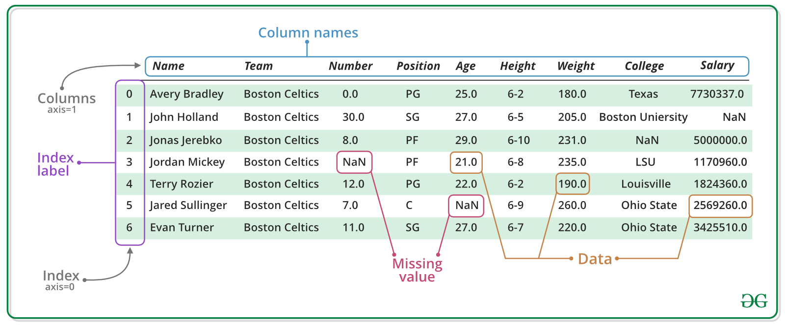
Series are limited to a single column. A more useful Pandas data structure is the DataFrame. A DataFrame is basically a bunch of series that share the same index.
data = {
    "capacity": [1269, 1365, 1290],  # MW
    "type": ["PWR", "PWR", "PWR"],
    "start_year": [1989, 1988, 1988],
    "end_year": [np.nan, np.nan, np.nan],
}
df = pd.DataFrame(data, index=["Neckarwestheim", "Isar 2", "Emsland"])
dfA wide range of statistical functions are available on both Series and DataFrames.
df.min()capacity 1269
type PWR
start_year 1988
end_year NaN
dtype: objectdf.mean(numeric_only=True)capacity 1308.000000
start_year 1988.333333
end_year NaN
dtype: float64We can get a single column as a Series using python’s getitem syntax on the DataFrame object.
df["capacity"]Neckarwestheim 1269
Isar 2 1365
Emsland 1290
Name: capacity, dtype: int64Indexing works very similar to series
df.loc["Emsland"]capacity 1290
type PWR
start_year 1988
end_year NaN
Name: Emsland, dtype: objectBut we can also specify the column(s) and row(s) we want to access
df.at["Emsland", "start_year"]np.int64(1988)We can also add new columns to the DataFrame:
df["reduced_capacity"] = df.capacity * 0.8
dfWe can also remove columns or rows from a DataFrame:
df.drop("reduced_capacity", axis="columns", inplace=True)We can also drop columns with only NaN values
df.dropna(axis=1)Or fill it up with default “fallback” data:
df.fillna(2023)Sorting Data
We can also sort the entries in dataframes, e.g. alphabetically by index or numerically by column values
df.sort_index()df.sort_values(by="capacity", ascending=False)Filtering Data
We can also filter a DataFrame using a boolean series obtained from a condition. This is very useful to build subsets of the DataFrame.
df.capacity > 1300Neckarwestheim False
Isar 2 True
Emsland False
Name: capacity, dtype: booldf[df.capacity > 1300]We can also combine multiple conditions, but we need to wrap the conditions with brackets!
df[(df.capacity > 1300) & (df.start_year >= 1988)]Or we make SQL-like queries:
df.query("start_year == 1988")threshold = 1300
df.query("start_year == 1988 and capacity > @threshold")Modifying Values
In many cases, we want to modify values in a dataframe based on some rule. To modify values, we need to use .loc or .iloc
df.loc["Isar 2", "capacity"] = 1366
dfSometimes it can be useful to rename columns:
df.rename(columns=dict(type="reactor"))Sometimes it can be useful to replace values:
df.replace({"PWR": "Pressurized water reactor"})Time Series
Time indexes are great when handling time-dependent data.
Let’s first read some time series data, using the pd.read_csv() function, which takes a local file path ora link to an online resource.
The example data hourly time series for Germany in 2015 for:
electricity demand from OPSD in GW
onshore wind capacity factors from renewables.ninja in per-unit of installed capacity
offshore wind capacity factors from renewables.ninja in per-unit of installed capacity
solar PV capacity factors from renewables.ninja in per-unit of installed capacity
electricity day-ahead spot market prices in €/MWh from EPEX Spot zone DE/AT/LU retrieved via SMARD platform
# Backup: https://cloud.pypsalabs.org/s/FSJ3qwQjqCxcWXQ/download/time-series-sample.csv
url = "https://raw.githubusercontent.com/pypsalabs/workshop-202609/main/bham/data/time-series-sample.csv"

ts = pd.read_csv(url, index_col=0, parse_dates=True)

ts.head()We can use Python’s slicing notation inside .loc to select a date range, and then use the built-in plotting feature of Pandas:
ts.loc["2015-01-01":"2015-03-01", "load"].plot()<Axes: >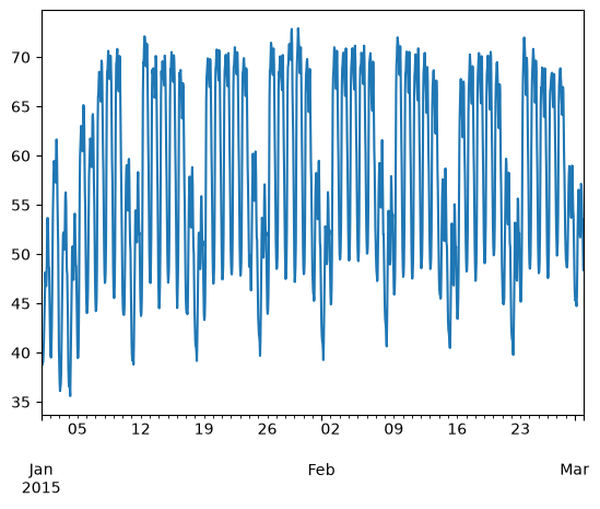
ts.loc["2015-05-01", "solar"].plot()<Axes: >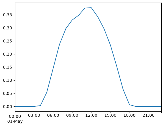
A common operation is to change the resolution of a dataset by resampling in time, which Pandas exposes through the resample function.
ts["onwind"].resample("ME").mean().plot()<Axes: >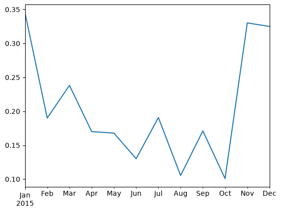
Groupby Functionality
DataFrame objects have a groupby method. The simplest way to think about it is that you pass another series, whose values are used to split the original object into different groups.
Here’s an example which retrieves the total generation capacity per country:
fn = "https://raw.githubusercontent.com/PyPSA/powerplantmatching/master/powerplants.csv"df = pd.read_csv(fn, index_col=0)
df.iloc[:5, :10]grouped = df.groupby("Country").Capacity.sum()
grouped.head()Country
Albania 2683.566000
Austria 27057.130368
Belgium 24244.510150
Bosnia and Herzegovina 5478.500000
Bulgaria 21015.140000
Name: Capacity, dtype: float64Let’s break apart this operation a bit. The workflow with groupby can be divided into three general steps:
Split: Partition the data into different groups based on some criterion.
Apply: Do some caclulation within each group, e.g. minimum, maximum, sums.
Combine: Put the results back together into a single object.
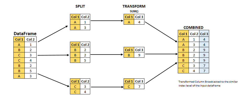
Grouping is not only possible on a single columns, but also on multiple columns. For instance,
we might want to group the capacities by country and fuel type. To achieve this, we pass a list of functions to the groupby functions.
capacities = df.groupby(["Country", "Fueltype"]).Capacity.sum()
capacities
Country Fueltype
Albania Hydro 2079.366
Solar 454.200
Wind 150.000
Austria Battery 40.320
Hard Coal 1471.000
...
United Kingdom Other 35.000
Solar 13679.900
Solid Biomass 4154.200
Waste 1948.150
Wind 39284.500
Name: Capacity, Length: 327, dtype: float64By grouping by multiple attributes, our index becomes a pd.MultiIndex (a hierarchical index with multiple levels.
capacities.index[:5]MultiIndex([('Albania', 'Hydro'),
('Albania', 'Solar'),
('Albania', 'Wind'),
('Austria', 'Battery'),
('Austria', 'Hard Coal')],
names=['Country', 'Fueltype'])We can use the .unstack function to reshape the multi-indexed pd.Series into a pd.DataFrame which has the second index level as columns.
capacities.unstack().tail().TExercises
Task 1: Provide a list of unique fuel types included in the power plants dataset.
Notebook Cell
df.Fueltype.unique()array(['Hydro', 'Hard Coal', 'Natural Gas', 'Lignite', 'Oil', 'Wind',
'Solid Biomass', 'Waste', 'Solar', 'Geothermal', 'Battery',
'Heat Storage', 'Nuclear', 'Other', 'Biogas', 'Mechanical Storage',
'Hydrogen Storage'], dtype=object)Task 2: Filter the dataset by power plants with the fuel type “Hard Coal”. How many hard coal power plants are there?
Notebook Cell
coal = df.loc[df.Fueltype == "Hard Coal"]
coalTask 3: Identify the three largest coal power plants. In which countries are they located? When were they built?
Notebook Cell
coal.loc[coal.Capacity.nlargest(3).index]Task 4: What is the average “DateIn” of each “Fueltype”? Which type of power plants is the oldest on average?
Notebook Cell
2024 - df.groupby("Fueltype").DateIn.mean().sort_values()Fueltype
Hard Coal 51.822630
Hydro 51.393134
Lignite 45.510067
Nuclear 43.344538
Other 23.950920
Geothermal 21.117647
Waste 20.210667
Oil 20.165703
Solid Biomass 17.119048
Wind 12.523960
Biogas 12.459045
Natural Gas 12.224814
Solar 6.951960
Battery 1.391788
Heat Storage NaN
Hydrogen Storage NaN
Mechanical Storage NaN
Name: DateIn, dtype: float64Task 5: In the time series provided, calculate the annual average capacity factors of wind and solar.
Notebook Cell
ts.mean()load 54.736992
onwind 0.205556
offwind 0.362993
solar 0.122621
prices 31.835717
dtype: float64Task 6: In the time series provided, calculate and plot the monthly average electricity price.
Notebook Cell
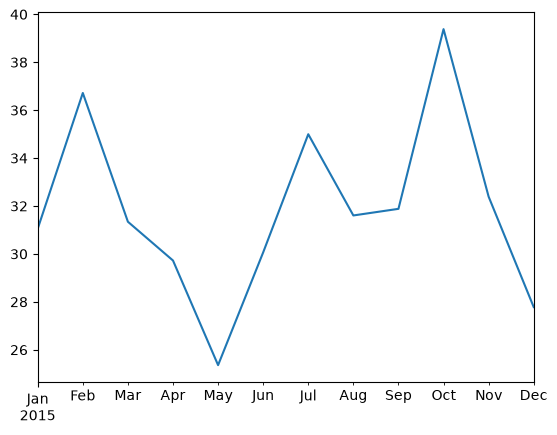
ts["prices"].resample("ME").mean().plot()<Axes: >