Introduction: PyPSA & linopy - PyPSA Workshop Birmingham

PyPSA is an open source Python package for simulating and optimising modern energy systems that include features such as

conventional generators with unit commitment (ramp-up, ramp-down, start-up, shut-down),
time-varying wind and solar generation,
energy storage with efficiency losses and inflow/spillage for hydroelectricity
coupling to other energy sectors (electricity, transport, heat, industry),
conversion between energy carriers (e.g. electricity to hydrogen),
transmission networks (AC, DC, other fuels)

PyPSA can be used for a variety of problem types (e.g. electricity market modelling, long-term investment planning, transmission network expansion planning), and is designed to scale well with large networks and long time series.

Compared to building power system by hand in linopy, PyPSA does the following things for you:

manage data inputs
build optimisation problem
communicate with the solver
retrieve and process optimisation results
manage data outputs

Dependencies¶

pandas for storing data about network components and time series
numpy and scipy for linear algebra and sparse matrix calculations
matplotlib and cartopy for plotting on a map
networkx for network calculations
linopy for handling optimisation problems

Note

On the workshop JupyterHub, everything is already installed - just log in and run the cells below, nothing to set up.

No hub access? You can also run this notebook in your browser on Google Colab (a Google account is required). On Colab, first run this in a cell at the top:

!pip install pypsa

Basic components¶

Component	Description
Network	Container for all components.
Bus	Node where components attach.
Carrier	Energy carrier or technology (e.g. electricity, hydrogen, gas, coal, oil, biomass, on-/offshore wind, solar). Can track properties such as specific carbon dioxide emissions or nice names and colors for plots.
Load	Energy consumer (e.g. electricity demand).
Generator	Generator (e.g. power plant, wind turbine, PV panel).
Line	Power distribution and transmission lines (overhead and cables).
Link	Links connect two buses with controllable energy flow, direction-control and losses. They can be used to model: HVDC links HVAC lines (neglecting KVL, only net transfer capacities (NTCs)) conversion between carriers (e.g. electricity to hydrogen in electrolysis)
StorageUnit	Storage with fixed nominal energy-to-power ratio.
Store	Storage with separately extendable energy capacity.
GlobalConstraint	Constraints affecting many components at once, such as emission limits.

Getting started¶

Simple electricity market problem¶

generator 1: “gas” -- marginal cost 70 EUR/MWh -- capacity 50 MW

generator 2: “nuclear” -- marginal cost 10 EUR/MWh -- capacity 100 MW

load: “Small town” -- demand 120 MW

single time step (“now”)

single node (“Springfield”)

Building a basic network¶

# By convention, PyPSA is imported without an alias:
import pypsa

# First, we create a network object which serves as the container for all components
n = pypsa.Network()

Empty PyPSA Network 'Unnamed Network'
-------------------------------
Components: none
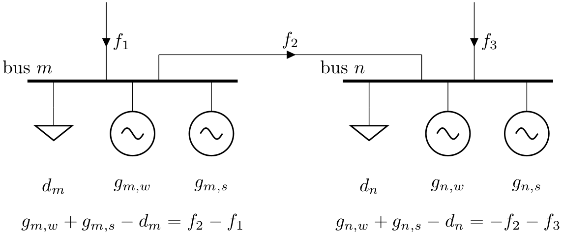
Snapshots: 1

The second component we need are buses. Buses are the fundamental nodes of the network, to which all other components like loads, generators and transmission lines attach. They enforce energy conservation for all elements feeding in and out of it (i.e. Kirchhoff’s Current Law).

Components can be added to the network n using the n.add() function. It takes the component name as a first argument, the name of the component as a second argument and possibly further parameters as keyword arguments. Let’s use this function to add a single bus, “Springfield”, to our network:

n.add("Bus", "Springfield", v_nom=380, carrier="AC")

For each class of components, the data describing the components is stored in a pandas.DataFrame. For example, all static data for buses is stored in n.buses

n.buses

You see there are many more attributes than we specified while adding the buses; many of them are filled with default parameters which were added. You can look up the field description, defaults and status (required input, optional input, output) for buses here https://docs.pypsa.org/latest/user-guide/components/buses/, and analogous for all other components.

The n.add() function lets you add any component to the network object n:

n.add(
    "Generator",
    "gas",
    bus="Springfield",
    p_nom_extendable=False,
    marginal_cost=70,  # €/MWh
    p_nom=50,  # MW
)
n.add(
    "Generator",
    "nuclear",
    bus="Springfield",
    p_nom_extendable=False,
    marginal_cost=10,  # €/MWh
    p_nom=100,  # MW
)

As a result, the n.generators DataFrame looks like this:

n.generators

Next, we’re going to add the electricity demand.

A positive value for p_set means consumption of power from the bus.

n.add(
    "Load",
    "Small town",
    bus="Springfield",
    p_set=120,  # MW
)

n.loads

Optimisation¶

The design principle of PyPSA is that basically each component is associated with a set of variables and constraints that will be added to the optimisation model based on the input data stored for the components.

For this dispatch problem, PyPSA will solve an optimisation problem that looks like this

\min_{g_{s,t};} \sum_{t,s} o_{s} g_{s,t}

(1)

such that

\begin{align} 0 & \leq g_{s,t} \leq G_{s} & \text{generation limits : generator} \\ D_t &= \sum_s g_{s,t} & \text{market clearing : bus} \\ \end{align}

(2)

Decision variables:

$g_{s,t}$ is the generator dispatch of technology $s$ at time $t$

Parameters:

$o_{s}$ is the marginal generation cost of technology $s$
$G_{s}$ is the nominal capacity of technology $s$
$D_t$ is the power demand in Springfield at time $t$

With all input data transferred into the PyPSA’s data structure (network), we can now build and run the resulting optimisation problem. In PyPSA, building, solving and retrieving results from the optimisation model is contained in a single function call n.optimize(). This function optimizes dispatch and investment decisions for least cost adhering to the constraints defined in the network.

The n.optimize() function can take a variety of arguments. The most relevant for the moment is the choice of the solver (e.g. “highs” and “gurobi”). They need to be installed on your computer, to use them here!

n.optimize(solver_name="highs")

/tmp/ipykernel_2501/3144390136.py:1: FutureWarning:

The default value of `include_objective_constant` will change from True to False in version 2.0. Set `include_objective_constant` explicitly to suppress this warning. Using False improves LP numerical conditioning by not including the objective constant as a variable.

WARNING:pypsa.consistency:The following buses have carriers which are not defined. Run n.sanitize() to add them. Components with undefined carriers:
Index(['Springfield'], dtype='object', name='name')

INFO:linopy.model: Solve problem using Highs solver

INFO:linopy.io: Writing time: 0.03s

INFO:linopy.constants: Optimization successful: 
Status: ok
Termination condition: optimal
Solution: 2 primals, 5 duals
Objective: 2.40e+03
Solver: highs
Runtime: 0.00s
MIP gap: inf
Dual bound: 0.00e+00
Solver model: available
Solver message: Optimal

INFO:pypsa.optimization.optimize:The shadow-prices of the constraints Generator-fix-p-lower, Generator-fix-p-upper were not assigned to the network.

Running HiGHS 1.15.1 (git hash: 04024d7): Copyright (c) 2026 under MIT licence terms
Includes third-party software components, see THIRD_PARTY_NOTICES.md for full details
LP linopy-problem-3tof75md has 5 rows; 2 cols; 6 nonzeros
Coefficient ranges:
  Matrix  [1e+00, 1e+00]
  Cost    [1e+01, 7e+01]
  Bound   [0e+00, 0e+00]
  RHS     [5e+01, 1e+02]
Presolving model
0 rows, 0 cols, 0 nonzeros 0s
0 rows, 0 cols, 0 nonzeros 0s
Presolve reductions: rows 0(-5); columns 0(-2); nonzeros 0(-6) - Reduced to empty
Performed postsolve
Solving the original LP from the solution after postsolve

Model name          : linopy-problem-3tof75md
Model status        : Optimal
Objective value     :  2.4000000000e+03
P-D objective error :  0.0000000000e+00
HiGHS run time      :          0.00

('ok', 'optimal')

Let’s have a look at the results. The network object n contains now the objective value and the results for the decision variables.

n.objective

2400.0

Since the power flow and dispatch are generally time-varying quantities, these are stored in a different locations than e.g. n.generators. They are stored in n.generators_t. Thus, to find out the dispatch of the generators, run

n.generators_t.p

n.buses_t.marginal_price

n.generators_t.mu_upper

Explore the PyPSA model¶

Under the hood, a call to n.optimize() builds a linopy optimisation model, solves it with the specified solver, and then retrieves the results back into the PyPSA data structure. We can access this intermediate linopy model via n.model. This allows us to explore the optimisation model in more detail, for instance to see all variables and constraints that were added to the optimisation problem.

n.model

Linopy LP model
===============

Variables:
----------
 * Generator-p (snapshot, name)

Expressions:
------------
<empty>

Constraints:
------------
 * Generator-fix-p-lower (snapshot, name)
 * Generator-fix-p-upper (snapshot, name)
 * Bus-nodal_balance (snapshot, name)

Status:
-------
ok

n.model.constraints

linopy.model.Constraints
------------------------
 * Generator-fix-p-lower (snapshot, name)
 * Generator-fix-p-upper (snapshot, name)
 * Bus-nodal_balance (snapshot, name)

n.model.constraints["Generator-fix-p-upper"]

Constraint `Generator-fix-p-upper` [snapshot: 1, name: 2]:
----------------------------------------------------------
[now, gas]: +1 Generator-p[now, gas]         ≤ 50.0
[now, nuclear]: +1 Generator-p[now, nuclear] ≤ 100.0

n.model.constraints["Bus-nodal_balance"]

Constraint `Bus-nodal_balance` [snapshot: 1, name: 1]:
------------------------------------------------------
[now, Springfield]: +1 Generator-p[now, gas] + 1 Generator-p[now, nuclear] = 120.0

n.model.objective

Objective:
----------
LinearExpression: +70 Generator-p[now, gas] + 10 Generator-p[now, nuclear]
Sense: min
Value: 2400.0

We can also retrieve the shadow prices (duals) of individual constraints, e.g. of the upper generation limits:

n.model.constraints["Generator-fix-p-upper"].dual.to_dataframe()

Let’s write optimization problem manually and reproduce the PyPSA model¶

PyPSA optimisation module is based on Linopy --- an open-source framework for formulating, solving, and analyzing optimization problems with Python.

With Linopy, you can create optimization models within Python that consist of decision variables, constraints, and optimization objectives. You can then solve these instances using a variety of commercial and open-source solvers (specialised software).

Linopy supports a wide range of problem types, including:

Linear programming
Integer programming
Mixed-integer programming
Quadratic programming

# remove all constraints
for name in list(n.model.constraints):
    n.model.remove_constraints(name)

n.model.constraints

linopy.model.Constraints
------------------------
<empty>

n.model.add_constraints(
    n.model["Generator-p"].sum(dim="name") == n.loads.p_set["Small town"],
    name="nodal_balance",
)

Constraint `nodal_balance` [snapshot: 1]:
-----------------------------------------
[now]: +1 Generator-p[now, gas] + 1 Generator-p[now, nuclear] = 120.0

n.model.add_constraints(n.model["Generator-p"].loc[:, "gas"] >= 0, name="p_lower_gas")

Constraint `p_lower_gas` [snapshot: 1]:
---------------------------------------
[now]: +1 Generator-p[now, gas] ≥ -0.0

n.model.add_constraints(
    n.model["Generator-p"].loc[:, "nuclear"] >= 0, name="p_lower_nuclear"
)

Constraint `p_lower_nuclear` [snapshot: 1]:
-------------------------------------------
[now]: +1 Generator-p[now, nuclear] ≥ -0.0

n.model.add_constraints(
    n.model["Generator-p"].loc[:, "gas"] <= n.generators.p_nom.loc["gas"],
    name="p_upper_gas",
)

Constraint `p_upper_gas` [snapshot: 1]:
---------------------------------------
[now]: +1 Generator-p[now, gas] ≤ 50.0

n.model.add_constraints(
    n.model["Generator-p"].loc[:, "nuclear"] <= n.generators.p_nom.loc["nuclear"],
    name="p_upper_nuclear",
)

Constraint `p_upper_nuclear` [snapshot: 1]:
-------------------------------------------
[now]: +1 Generator-p[now, nuclear] ≤ 100.0

# check that we did a good job
n.model.constraints

linopy.model.Constraints
------------------------
 * nodal_balance (snapshot)
 * p_lower_gas (name, snapshot)
 * p_lower_nuclear (name, snapshot)
 * p_upper_gas (name, snapshot)
 * p_upper_nuclear (name, snapshot)

Let’s ensure that we get the same results as when using the n.optimize() function

n.optimize.solve_model(solver_name="highs")

INFO:linopy.model: Solve problem using Highs solver

INFO:linopy.io: Writing time: 0.03s

INFO:linopy.constants: Optimization successful: 
Status: ok
Termination condition: optimal
Solution: 2 primals, 10 duals
Objective: 2.40e+03
Solver: highs
Runtime: 0.00s
MIP gap: inf
Dual bound: 0.00e+00
Solver model: available
Solver message: Optimal

INFO:pypsa.optimization.optimize:The shadow-prices of the constraints nodal_balance, p_lower_gas, p_lower_nuclear, p_upper_gas, p_upper_nuclear were not assigned to the network.

Running HiGHS 1.15.1 (git hash: 04024d7): Copyright (c) 2026 under MIT licence terms
Includes third-party software components, see THIRD_PARTY_NOTICES.md for full details
LP linopy-problem-vy6ogdhy has 5 rows; 2 cols; 6 nonzeros
Coefficient ranges:
  Matrix  [1e+00, 1e+00]
  Cost    [1e+01, 7e+01]
  Bound   [0e+00, 0e+00]
  RHS     [5e+01, 1e+02]
Presolving model
0 rows, 0 cols, 0 nonzeros 0s
0 rows, 0 cols, 0 nonzeros 0s
Presolve reductions: rows 0(-5); columns 0(-2); nonzeros 0(-6) - Reduced to empty
Performed postsolve
Solving the original LP from the solution after postsolve

Model name          : linopy-problem-vy6ogdhy
Model status        : Optimal
Objective value     :  2.4000000000e+03
P-D objective error :  0.0000000000e+00
HiGHS run time      :          0.00

('ok', 'optimal')

n.generators_t.p

n.model

Linopy LP model
===============

Variables:
----------
 * Generator-p (snapshot, name)

Expressions:
------------
<empty>

Constraints:
------------
 * nodal_balance (snapshot)
 * p_lower_gas (name, snapshot)
 * p_lower_nuclear (name, snapshot)
 * p_upper_gas (name, snapshot)
 * p_upper_nuclear (name, snapshot)

Status:
-------
ok

Making use of Expressions¶

Besides variables and constraints, a linopy model has a third group: Expressions. These are named linear expressions, i.e. combinations of variables that are not (yet) turned into a constraint or an objective.

Registering an expression with n.model.add_expressions(..., name=...) makes it part of the model:

it appears in the model summary,
it can be reused when building further expressions, constraints or the objective,
after solving, it evaluates to numbers via .solution.

This is handy for derived quantities you want to report, without recomputing them by hand from the decision variables.

# total dispatch per snapshot, dims: (snapshot)
total_generation = n.model.add_expressions(
    n.model["Generator-p"].sum(dim="name"), name="total_generation"
)
total_generation

LinearExpression [snapshot: 1]:
-------------------------------
[now]: +1 Generator-p[now, gas] + 1 Generator-p[now, nuclear]

# operational cost; a scalar expression that should coincide with the objective
operational_cost = n.model.add_expressions(
    (n.generators.marginal_cost * n.model["Generator-p"]).sum(), name="operational_cost"
)
operational_cost

LinearExpression
----------------
+70 Generator-p[now, gas] + 10 Generator-p[now, nuclear]

# the Expressions group is no longer empty. Expressions have no numerical value until the model is solved.
n.model

Linopy LP model
===============

Variables:
----------
 * Generator-p (snapshot, name)

Expressions:
------------
 * total_generation (snapshot)
 * operational_cost

Constraints:
------------
 * nodal_balance (snapshot)
 * p_lower_gas (name, snapshot)
 * p_lower_nuclear (name, snapshot)
 * p_upper_gas (name, snapshot)
 * p_upper_nuclear (name, snapshot)

Status:
-------
ok

n.model.solve(solver_name="highs")

INFO:linopy.model: Solve problem using Highs solver

INFO:linopy.io: Writing time: 0.03s

INFO:linopy.constants: Optimization successful: 
Status: ok
Termination condition: optimal
Solution: 2 primals, 10 duals
Objective: 2.40e+03
Solver: highs
Runtime: 0.00s
MIP gap: inf
Dual bound: 0.00e+00
Solver model: available
Solver message: Optimal

Running HiGHS 1.15.1 (git hash: 04024d7): Copyright (c) 2026 under MIT licence terms
Includes third-party software components, see THIRD_PARTY_NOTICES.md for full details
LP linopy-problem-rv6ditti has 5 rows; 2 cols; 6 nonzeros
Coefficient ranges:
  Matrix  [1e+00, 1e+00]
  Cost    [1e+01, 7e+01]
  Bound   [0e+00, 0e+00]
  RHS     [5e+01, 1e+02]
Presolving model
0 rows, 0 cols, 0 nonzeros 0s
0 rows, 0 cols, 0 nonzeros 0s
Presolve reductions: rows 0(-5); columns 0(-2); nonzeros 0(-6) - Reduced to empty
Performed postsolve
Solving the original LP from the solution after postsolve

Model name          : linopy-problem-rv6ditti
Model status        : Optimal
Objective value     :  2.4000000000e+03
P-D objective error :  0.0000000000e+00
HiGHS run time      :          0.00

('ok', 'optimal')

# all registered expressions evaluated at the optimum, as one xarray.Dataset
n.model.expressions.solution.to_pandas()

# or one at a time; the cost expression reproduces the objective value
n.model.expressions["operational_cost"].solution.item() == n.model.objective.value

True

Component objects in PyPSA v1¶

Since PyPSA v1.0, every component type also has a dedicated Components object, available through n.components or its short alias n.c. The Components class adds functionality beyond raw DataFrames, including shared methods and properties on pypsa.Components and features specific to individual component types.

The underlying pandas-based data structure remains unchanged. Each component object provides access to two stores:

.static: one row per asset for values that do not vary across snapshots, such as nominal capacity or marginal cost;
.dynamic: a dictionary-like collection of time-indexed DataFrames, such as dispatch or marginal prices.

These are exactly the same data exposed by the familiar plural and _t accessors. For example, n.components.generators.static is n.generators, while n.components.generators.dynamic is n.generators_t. Both styles are supported in PyPSA v1.

# Access the Generators component object, which bundles component data and functionality
generators = n.components.generators
generators

'Generator' Components
----------------------
Attached to PyPSA Network 'Unnamed Network'
Components: 2

# Access time-dependent dispatch through the familiar `_t` accessor
n.generators_t.p

# Access the same dispatch DataFrame through the Components API
generators.dynamic.p

# Confirm that both accessors point to the exact same DataFrame, not a copy
n.generators_t.p is n.components.generators.dynamic.p

True

# Select static generator attributes, with one row per asset
generators.static[["bus", "p_nom", "marginal_cost"]]

# Inspect which generators are extendable and which have fixed capacities
print(generators.extendables)
print(generators.fixed)

Index([], dtype='object', name='name')
Index(['gas', 'nuclear'], dtype='object', name='name')