Stochastic & Risk-Averse Optimization - PyPSA Workshop Birmingham

Note

On the workshop JupyterHub, everything is already installed - just log in and run the cells below, nothing to set up.

No hub access? You can also run this notebook in your browser on Google Colab (a Google account is required). On Colab, first run this in a cell at the top:

!pip install pypsa "plotly<6"

Achieving climate-neutral energy systems requires bulky and expensive infrastructure investments taken now under deep uncertainty — from fuel price shocks and geopolitical disruptions to extreme weather and technology surprises. Investment plans carry risks, but must remain viable and resilient across all plausible futures.

In this tutorial, we explore how PyPSA can help you plan rationally when the future is unknown. We will focus on:

Exploring why single-scenario plans are fragile,
Running and interpreting stochastic optimisation in PyPSA, including value-of-information metrics (EVPI & VSS),
Evaluating trade-offs between expected cost and worst-case risk with Conditional Value at Risk (CVaR).

See also User Guide — Stochastic Optimisation in the PyPSA documentation.

import logging

import pandas as pd
import plotly.express as px
import plotly.graph_objects as go
import pypsa

pypsa.options.params.optimize.include_objective_constant = False
pypsa.options.params.optimize.log_to_console = False

# hide a harmless linopy performance warning emitted for stochastic networks
logging.getLogger("linopy.expressions").setLevel(logging.ERROR)

A toy capacity expansion model¶

As a playground, we use the single-node capacity expansion model from model.energy, which is shipped with PyPSA as an example network. It optimises investment and dispatch of wind, solar, battery storage and hydrogen storage (electrolysis, steel tank storage, turbine) to serve an electricity demand averaging 7.6 GW, based on a year of real demand and weather time series. We make two additions:

a fossil backup generator (efficiency 0.4, marginal cost 100 €/MWh, annualised capital cost 100 k€/MW/a),
a higher load shedding cost of 10,000 €/MWh (the value of lost load).

In very stylised form, the model solves a linear optimisation problem to find the least-cost investment and dispatch plan:

\begin{aligned} \min \quad & \text{CAPEX} + \sum_t \text{OPEX}_t \\ \text{s.t.} \quad & \text{dispatch}_{\text{tech},t} \leq \text{capacity}_{\text{tech}} && \forall\, t, \text{tech} \\ & \sum_{\text{tech}} \text{dispatch}_{\text{tech},t} = \text{demand}_t && \forall\, t \end{aligned}

(1)

…plus renewable availability, storage operation and load shedding constraints across all hours of the year. To keep solving times classroom-friendly, we resample the time series from 3-hourly to 6-hourly resolution.

def prepare_network():
    """Build the model.energy example extended by a fossil backup generator."""
    n = pypsa.examples.model_energy()
    n.add(
        "Generator",
        "fossil backup",
        carrier="fossil backup",
        bus="electricity",
        p_nom_extendable=True,
        efficiency=0.4,
        marginal_cost=100,
        capital_cost=100_000,
    )
    n.add("Carrier", "fossil backup", color="indianred")
    n.generators.loc["load shedding", "marginal_cost"] = 10_000
    return n.cluster.temporal.resample("6h")


base = prepare_network()
base.generators[["p_nom_extendable", "capital_cost", "marginal_cost", "efficiency"]]

Deterministic plans for three futures¶

We live in an era of compounding uncertainties: fuel price crises, volcanic eruptions dimming the sun, cost forecasts arriving early or late, droughts, sabotage. Let us focus on three illustrative futures:

Scenario	Story	Parameter change	Probability
baseline	default assumptions	—	50%
gas crisis	fuel supply disruption	fossil backup marginal cost ×5	40%
volcano	eruption dims the sky	solar availability ×0.1	10%

The classical planning approach is to optimise the system for each scenario separately, assuming perfect foresight. The probabilities come into play later.

PROB = {"baseline": 0.5, "gas crisis": 0.4, "volcano": 0.1}
GAS_PRICE = {"baseline": 100, "gas crisis": 500, "volcano": 100}  # €/MWh
SOLAR_FACTOR = {"baseline": 1.0, "gas crisis": 1.0, "volcano": 0.1}
SCENARIOS = list(PROB)


def apply_scenario(n, scenario):
    """Set the fossil fuel price and solar availability of a scenario."""
    n.generators.at["fossil backup", "marginal_cost"] = GAS_PRICE[scenario]
    n.generators_t.p_max_pu["solar"] = (
        base.generators_t.p_max_pu["solar"] * SOLAR_FACTOR[scenario]
    )

plans = {}
for s in SCENARIOS:
    n = base.copy()
    apply_scenario(n, s)
    n.optimize()
    plans[s] = n

pd.concat(
    {s: n.statistics.optimal_capacity() for s, n in plans.items()}, axis=1
).fillna(0).round(0)

The three plans differ substantially: the gas crisis plan builds much more wind, solar and storage — including a large hydrogen storage system — to avoid burning expensive fuel, while the volcano plan builds no solar at all and relies on wind and fossil backup instead.

Let’s compare the total system costs of the three plans, split into annualised investment costs per technology plus the operating costs (fuel and load shedding).

COLORS = {
    "wind": "dodgerblue",
    "solar": "gold",
    "battery storage": "palegreen",
    "hydrogen storage": "orchid",
    "fossil backup": "indianred",
    "fuel cost": "lightcoral",
    "load shedding": "dimgray",
}


def cost_breakdown(n):
    """Cost components in bn€/a, per scenario if the network is stochastic."""
    groups = {"electrolysis": "hydrogen storage", "turbine": "hydrogen storage"}
    capex = n.statistics.capex().rename(groups, level="carrier")
    opex = n.statistics.opex().rename({"fossil backup": "fuel cost"}, level="carrier")
    costs = pd.concat([capex, opex]).div(1e9)
    levels = [lv for lv in ["scenario", "carrier"] if lv in costs.index.names]
    return costs.groupby(level=levels).sum()


plan_costs = (
    pd.concat({s: cost_breakdown(n) for s, n in plans.items()}, names=["plan"])
    .rename("cost")
    .reset_index()
)

fig = px.bar(
    plan_costs,
    x="plan",
    y="cost",
    color="carrier",
    color_discrete_map=COLORS,
    category_orders={"carrier": list(COLORS), "plan": SCENARIOS},
    labels={"cost": "total system cost [bn€/a]"},
    title="Optimal plans for each scenario",
    width=600,
    height=450,
)
fig

So we obtain a different least-cost strategy for each future. But these costs are only valid if the planned-for scenario actually arrives.

How would you decide which strategy to implement? And what happens if the wrong scenario arrives?

Every plan has an Achilles heel¶

Investments are long-lived: once built, the capacities are locked in, and only the dispatch can adapt to whatever future materialises. To stress-test a plan, we therefore fix its optimal capacities (n.optimize.fix_optimal_capacities()) and re-optimise the dispatch under each of the other scenarios.

def evaluate(plan, scenario):
    """Re-dispatch the fixed capacities of `plan` under a different `scenario`."""
    plan.model.solver_model = None  # required before copying a solved network
    m = plan.copy()
    m.optimize.fix_optimal_capacities()
    apply_scenario(m, scenario)
    m.optimize()
    return m


outcomes = {
    (p, s): plans[p] if p == s else evaluate(plans[p], s)
    for p in SCENARIOS
    for s in SCENARIOS
}

det_costs = (
    pd.concat(
        {k: cost_breakdown(m) for k, m in outcomes.items()},
        names=["plan", "outcome"],
    )
    .rename("cost")
    .reset_index()
)

# first bar of each panel: the plan's cost as planned (its own scenario)
plan_bars = det_costs.query("plan == outcome").assign(outcome="Plan")

capex_total = {s: plans[s].statistics.capex().sum() / 1e9 for s in SCENARIOS}

BAR_LABEL = {"Plan": "Plan", **{s: s.title() + "<br>Outcome" for s in SCENARIOS}}


def outcome_figure(df, plan_order, capex, title):
    """Faceted stacked cost bars per plan: planned cost, then re-dispatched outcomes."""
    fig = px.bar(
        df.assign(outcome=df["outcome"].map(BAR_LABEL)),
        x="outcome",
        y="cost",
        color="carrier",
        facet_col="plan",
        color_discrete_map=COLORS,
        category_orders={
            "carrier": list(COLORS),
            "plan": plan_order,
            "outcome": list(BAR_LABEL.values()),
        },
        labels={"cost": "total system cost [bn€/a]", "outcome": ""},
        title=title,
        height=500,
    )
    for i, p in enumerate(plan_order, start=1):
        fig.add_hline(y=capex[p], row=1, col=i, line_dash="dot", line_color="gray")
        fig.add_vline(x=0.5, row=1, col=i, line_dash="dot", line_color="gray")
    fig.add_scatter(
        x=[None],
        y=[None],
        mode="lines",
        line={"dash": "dot", "color": "gray"},
        name="CAPEX",
    )
    fig.for_each_annotation(lambda a: a.update(text=a.text.split("=", 1)[1]))
    fig.update_layout(legend={"orientation": "h", "title": None, "y": -0.3})
    return fig


outcome_figure(
    pd.concat([plan_bars, det_costs]),
    SCENARIOS,
    capex_total,
    "Each plan as planned and re-dispatched under each outcome",
)

All strategies perform poorly in at least one scenario they were not planned for: the baseline plan costs 12.3 bn€/a if the gas crisis hits (up from 5.4), and the solar-free volcano plan explodes to 17.1 bn€/a in a gas crisis: having built neither solar nor meaningful storage, it burns expensive fuel whenever wind is low. The dotted lines mark the CAPEX, which is fixed across outcomes — only the operating costs react to the scenario.

Now the probabilities from our scenario table come into play. We use them to compute the expected total cost of each plan across all possible outcomes.

tsc = (
    det_costs.groupby(["plan", "outcome"])["cost"]
    .sum()
    .unstack("outcome")
    .loc[SCENARIOS, SCENARIOS]
)
probs = pd.Series(PROB)
expected = (tsc @ probs).rename("expected cost [bn€/a]")
expected.to_frame().style.background_gradient(
    cmap="Blues", vmax=float(expected.max()) * 2
).format("{:.2f}")

The gas crisis plan has the lowest expected cost (7.7 bn€/a) — but uncertainty was never considered in the planning itself, and a risk of high costs is present in every plan.

Which strategy would you choose and why? And can we do better than picking one of the three?

Stochastic optimisation¶

Two-stage stochastic programming finds the single plan that minimises the expected total cost across all scenarios:

\begin{aligned} \min \quad & \overbrace{\text{CAPEX}}^{\substack{\text{here-and-now}\\\text{first-stage decisions}}} + \sum_{s} p_s \sum_t \overbrace{\text{OPEX}_{t,s}}^{\substack{\text{wait-and-see}\\\text{second-stage decisions}}} \\ \text{s.t.} \quad & \text{dispatch}_{\text{tech},t,s} \leq \text{capacity}_{\text{tech}} && \forall\, t, \text{tech}, s \\ & \sum_{\text{tech}} \text{dispatch}_{\text{tech},t,s} = \text{demand}_{t,s} && \forall\, t, s \end{aligned}

(2)

where $p_s$ is the probability of scenario $s$ . Investment decisions are made before the uncertainty resolves and are shared by all scenarios; dispatch decisions adapt to each scenario afterwards.

In PyPSA, n.set_scenarios() transforms a network into a stochastic network by adding a scenario dimension to all component data, so that scenario-specific parameters can be set directly.

n_stoch = base.copy()
n_stoch.set_scenarios(PROB)

n_stoch.generators.at[("gas crisis", "fossil backup"), "marginal_cost"] = GAS_PRICE[
    "gas crisis"
]
n_stoch.generators_t.p_max_pu.loc[:, ("volcano", "solar")] *= SOLAR_FACTOR["volcano"]

n_stoch.generators.marginal_cost.xs("fossil backup", level="name")

scenario
baseline      100.0
gas crisis    500.0
volcano       100.0
Name: marginal_cost, dtype: float64

n_stoch.optimize()

print(f"Expected total system cost: {n_stoch.objective / 1e9:.2f} bn€/a")

Expected total system cost: 7.15 bn€/a

How does the stochastic plan compare to the three deterministic plans? In the figure below, the first bar of each panel shows the plan’s cost as planned — for the stochastic plan, that is its expected cost across the three scenarios.

capacities = {s: n.statistics.optimal_capacity() for s, n in plans.items()}
capacities["stochastic"] = n_stoch.statistics.optimal_capacity().xs(
    "baseline", level="scenario"
)

pd.concat(capacities, axis="columns").fillna(0).round()

def stochastic_costs(n, name):
    """Tidy cost rows: the expected-cost "Plan" bar plus each scenario outcome."""
    bd = cost_breakdown(n)
    plan = (
        bd.mul(n.scenario_weightings.weight, level="scenario")
        .groupby(level="carrier")
        .sum()
    )
    rows = pd.concat(
        [
            plan.rename("cost").reset_index().assign(outcome="Plan"),
            bd.rename("cost").reset_index().rename(columns={"scenario": "outcome"}),
        ]
    )
    return rows.assign(plan=name)


stoch_costs = stochastic_costs(n_stoch, "stochastic")
capex_total["stochastic"] = (
    n_stoch.statistics.capex().xs("baseline", level="scenario").sum() / 1e9
)

outcome_figure(
    pd.concat([plan_bars, det_costs, stoch_costs]),
    [*SCENARIOS, "stochastic"],
    capex_total,
    "Deterministic plans vs. the stochastic plan",
)

tsc_stoch = cost_breakdown(n_stoch).groupby("scenario").sum()
sp = tsc_stoch @ probs  # expected cost of the stochastic plan

expected_all = pd.concat([expected, pd.Series({"stochastic": sp})]).rename(
    "expected cost [bn€/a]"
)
expected_all.to_frame().style.background_gradient(
    cmap="Blues", vmax=float(expected_all.max()) * 2
).format("{:.2f}")

The stochastic plan reduces the expected cost to 7.15 bn€/a — about 7% below the best deterministic plan.

However, substantial risk remains in the low-probability volcano event. The reason: by minimising expected costs, the stochastic plan is risk-neutral — even though investors and planners are typically risk-averse. We come back to this after a short detour.

The value of information¶

Two classic metrics quantify what stochastic optimisation buys us (Birge & Louveaux, 2011):

For each scenario $s$ , let $z_s^{\mathrm{PI}}$ be the unweighted optimal cost when that scenario is known in advance. The wait-and-see value is their probability-weighted average, $\mathrm{WS} = \sum_s p_s z_s^{\mathrm{PI}}$ . The expected value of perfect information $\mathrm{EVPI} = \mathrm{SP} - \mathrm{WS}$ is the most we should ever pay for a perfect forecast, where SP is the expected cost of the stochastic plan.
The expected-value plan ignores uncertainty and optimises for the average scenario. Evaluating its fixed capacities under each scenario gives the $\text{EEV}$ , and the value of the stochastic solution $\text{VSS} = \text{EEV} - \text{SP}$ is the gain from modelling uncertainty explicitly rather than averaging it away (Birge, 1982).

ws = sum(PROB[s] * tsc.at[s, s] for s in SCENARIOS)
evpi = sp - ws

print(f"WS   = {ws:.2f} bn€/a")
print(f"SP   = {sp:.2f} bn€/a")
print(f"EVPI = {evpi:.2f} bn€/a")

WS   = 6.34 bn€/a
SP   = 7.15 bn€/a
EVPI = 0.81 bn€/a

n_ev = base.copy()
n_ev.generators.at["fossil backup", "marginal_cost"] = sum(
    PROB[s] * GAS_PRICE[s] for s in SCENARIOS
)
n_ev.generators_t.p_max_pu["solar"] *= sum(PROB[s] * SOLAR_FACTOR[s] for s in SCENARIOS)
n_ev.optimize()

eev = sum(PROB[s] * cost_breakdown(evaluate(n_ev, s)).sum() for s in SCENARIOS)
vss = eev - sp

print(f"EEV  = {eev:.2f} bn€/a")
print(f"VSS  = {vss:.2f} bn€/a")

EEV  = 7.35 bn€/a
VSS  = 0.20 bn€/a

The ordering $\text{WS} \leq \text{SP} \leq \text{EEV}$ always holds. Here, a perfect forecast would be worth up to 0.81 bn€/a (EVPI, about 11% of system cost), while simply averaging the scenarios instead of modelling them costs an extra 0.20 bn€/a per year (VSS).

Risk aversion with CVaR¶

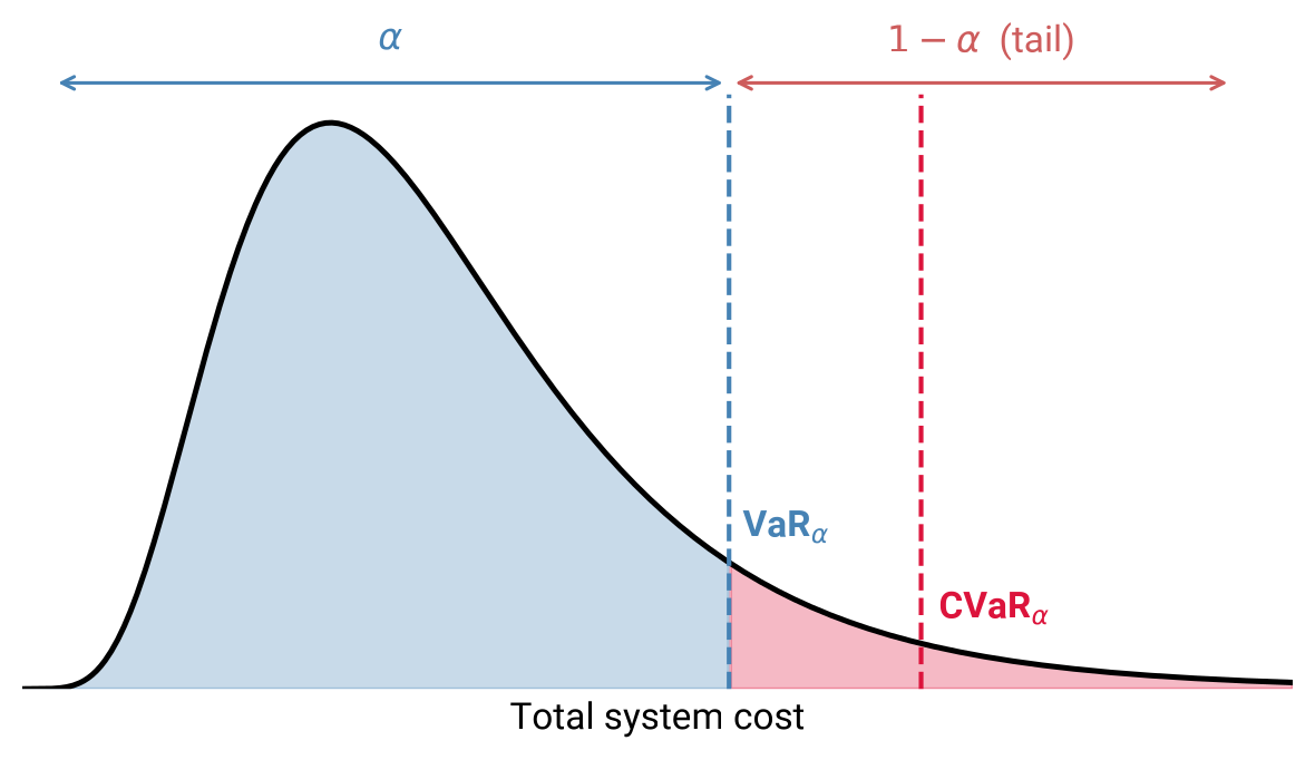
The stochastic plan minimises expected costs, giving a 10%-probability event only 10% weight — no matter how catastrophic it is. Risk-averse planners accept a higher expected cost to suppress such worst-case outcomes.

Conditional Value at Risk (CVaR) is a risk measure from finance (Rockafellar & Uryasev, 2002) that captures the expected cost in the worst-case tail of the cost distribution:

\text{CVaR}_{\alpha} = \mathbb{E}\left[\text{OPEX}_s \mid \text{OPEX}_s \geq \text{VaR}_{\alpha}\right]

(3)

where the value at risk $\text{VaR}_{\alpha}$ is the cost at the $\alpha$ -quantile, i.e. the threshold to the worst $(1-\alpha)$ share of outcomes:

Value at Risk marks the tail threshold; Conditional Value at Risk is the expected cost within that tail.

Adding CVaR to the objective, the parameter $\omega$ linearly shifts weight from the expected cost to the tail cost:

\min \quad \underbrace{\text{CAPEX}}_{\text{common investments}} + \underbrace{(1-\omega) \sum_{s} p_s \, \text{OPEX}_s}_{\text{risk-neutral fraction}} + \underbrace{\omega \cdot \text{CVaR}_{\alpha}}_{\text{risk-averse fraction}}

(4)

The user controls which outcomes count as the tail with $\alpha$ and how much the tail matters with $\omega \in [0, 1]$ ; the worst case itself is identified internally by the optimisation, which remains a linear program. The auxiliary variables and constraints behind this linearisation are described in the PyPSA stochastic optimisation docs.

With $\alpha = 0.9$ and our probabilities, the 10% tail is exactly the worst-performing scenario — whichever one that turns out to be. In PyPSA, this only takes n.set_risk_preference():

ALPHA = 0.9


def risk_variant(omega):
    """Copy of the stochastic network solved with risk preference (ALPHA, omega)."""
    n_stoch.model.solver_model = None
    m = n_stoch.copy()
    m.set_risk_preference(alpha=ALPHA, omega=omega)
    m.optimize()
    return m


n_mixed = risk_variant(omega=0.5)
n_averse = risk_variant(omega=1.0)

risk_nets = {
    "Planned with ω = 0<br>(risk-neutral)": n_stoch,
    "Planned with ω = 0.5, α = 0.9<br>(mixed)": n_mixed,
    "Planned with ω = 1, α = 0.9<br>(risk-averse)": n_averse,
}

risk_costs = pd.concat([stochastic_costs(n, name) for name, n in risk_nets.items()])
risk_capex = {
    name: n.statistics.capex().xs("baseline", level="scenario").sum() / 1e9
    for name, n in risk_nets.items()
}

outcome_figure(
    risk_costs,
    list(risk_nets),
    risk_capex,
    "How risk aversion (ω) affects the plan and its outcomes",
)

Higher risk aversion hedges against risky scenarios by shifting costs from the tail (OPEX) to upfront investments (CAPEX) note the rising dotted lines: more wind and hydrogen storage is built so that less fuel is burned when things go wrong. Increasing $\omega$ progressively levels out the cost differences across scenarios: at $\omega = 1$ , all three outcomes cost the same 7.97 bn€/a — but the expected cost has risen from 7.15 to 7.97 bn€/a.

The cost-risk frontier¶

So which $\omega$ should a planner choose? Sweeping $\omega$ from 0 to 1 traces out the available trade-offs between two quantities:

the insurance premium — the additional expected cost of a hedging strategy compared to the risk-neutral plan, and
the tail risk reduction — the decrease in CVaR it achieves.

Since our 10% tail is exactly the worst scenario, the CVaR here simply equals the highest operating cost across scenarios.

def risk_metrics(n):
    """Expected total cost and CVaR (tail operating cost) in bn€/a."""
    exp_cost = cost_breakdown(n).groupby("scenario").sum() @ probs
    tail_opex = n.statistics.opex().div(1e9).groupby("scenario").sum().max()
    return {"expected cost": exp_cost, "CVaR": tail_opex}


frontier = {
    0.0: risk_metrics(n_stoch),
    0.5: risk_metrics(n_mixed),
    1.0: risk_metrics(n_averse),
}
for omega in [0.05, 0.1, 0.2, 0.3, 0.7]:
    frontier[omega] = risk_metrics(risk_variant(omega))

fr = pd.DataFrame(frontier).T.sort_index()
fr["premium"] = fr["expected cost"] - fr["expected cost"].min()
fr.round(3)

fig = go.Figure(
    go.Scatter(
        x=fr["premium"],
        y=fr["CVaR"],
        mode="lines+markers",
        line={"color": "lightgray", "dash": "dot"},
        marker={
            "color": fr.index * 100,
            "colorscale": "Plasma",
            "size": 12,
            "colorbar": {"title": "risk aversion ω [%]"},
        },
    )
)
fig.update_layout(
    title="Tail risk reduction vs. insurance premium",
    xaxis_title="insurance premium [bn€/a]",
    yaxis_title="CVaR (tail operating cost) [bn€/a]",
    width=700,
    height=450,
)
fig

The frontier is strongly convex, meaning that the first steps of hedging come almost for free. For a premium of only 0.02 bn EUR per year ( $\omega = 0.3$ ), the tail cost already drops from 2.63 to 2.30 bn EUR per year. Eliminating the last bit of risk ( $\omega = 1$ ), in contrast, requires a premium of 0.82 bn EUR per year.

Which level of risk aversion would you choose — as a national planner? As a private investor? And why?

Summary¶

Deterministic single-scenario plans are fragile, ie each is optimal for one future and can be costly in the others.
Stochastic optimisation finds a single plan hedging across uncertain futures by minimising the expected cost.
CVaR embeds risk preferences and suppresses tail costs. Risk-averse investors pay more upfront to avoid worst-case outcomes.
The cost-risk frontier illustrates how small insurance premium buys a large tail risk reduction.

Exercises¶

Task 1: Volcanologists revise their assessment: the eruption probability rises to 30% (baseline drops to 30%). Rebuild the stochastic plan. How do the optimal capacities, scenario costs and expected cost change?

Task 2: Re-solve the risk-averse plan with alpha=0.6 and omega=1. The 40% tail now covers more than the single worst scenario. Compare the resulting capacities and scenario costs with the alpha=0.9 plan.

References¶

Birge, J. R., & Louveaux, F. (2011). Introduction to Stochastic Programming. In Springer Series in Operations Research and Financial Engineering. Springer New York. 10.1007/978-1-4614-0237-4
Birge, J. R. (1982). The value of the stochastic solution in stochastic linear programs with fixed recourse. Mathematical Programming, 24(1), 314–325. 10.1007/bf01585113
Rockafellar, R. T., & Uryasev, S. (2002). Conditional value-at-risk for general loss distributions. Journal of Banking & Finance, 26(7), 1443–1471. 10.1016/s0378-4266(02)00271-6