Recap: basic components
| Component | Description |
|---|---|
| Network | Container for all components. |
| Bus | Node where components attach. |
| Carrier | Energy carrier or technology (e.g. electricity, hydrogen, gas, coal, oil, biomass, on-/offshore wind, solar). Can track properties such as specific carbon dioxide emissions or nice names and colors for plots. |
| Load | Energy consumer (e.g. electricity demand). |
| Generator | Generator (e.g. power plant, wind turbine, PV panel). |
| Line | Power distribution and transmission lines (overhead and cables). |
| Link | Links connect two buses with controllable energy flow, direction-control and losses. They can be used to model:
|
| StorageUnit | Storage with fixed nominal energy-to-power ratio. |
| Store | Storage with separately extendable energy capacity. |
| GlobalConstraint | Constraints affecting many components at once, such as emission limits. |
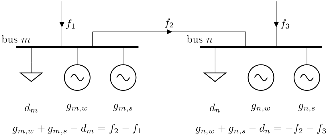
A more general form of an electricity dispatch problem
For an hourly electricity market dispatch simulation, PyPSA will solve an optimisation problem that looks like this
such that
Decision variables:
is the generator dispatch at bus , technology , time step ,
is the power flow in line ,
denotes the charge and discharge of storage unit at bus and time step ,
is the state of charge of storage at bus and time step .
Parameters:
is the marginal generation cost of technology at bus ,
is the reactance of transmission line ,
is the incidence matrix,
is the cycle matrix,
is the nominal capacity of the generator of technology at bus ,
is the rating of the transmission line ,
is the energy capacity of storage at bus ,
denote the standing (0), charging (1), and discharging (2) efficiencies.
South Africa & Mozambique system example
Compared to the previous example, we will consider a more complex system with more components (generators, transmission lines) and more buses. We also discuss basics of the plotting functionality built into PyPSA.
We have the following data:
fuel costs in € / MWh
fuel_cost = {
    "coal": 8,
    "gas": 100,
    "oil": 48,
}
efficiencies of thermal power plants in MWh / MWh
efficiency = {
    "coal": 0.33,
    "gas": 0.58,
    "oil": 0.35,
}
specific emissions in t / MWh
# t/MWh thermal
emissions = {
    "coal": 0.34,
    "gas": 0.2,
    "oil": 0.26,
    "hydro": 0,
    "wind": 0,
}
power plant capacities in MW
power_plants = {
    "SA": {"coal": 35000, "wind": 3000, "gas": 8000, "oil": 2000},
    "MZ": {"hydro": 1200},
}
electrical load in MW
loads = {
    "SA": 42000,
    "MZ": 650,
}
Building the network
By convention, PyPSA is imported without an alias:
import pypsa

pypsa.options.params.optimize.include_objective_constant = False
First, we create a new network object which serves as the overall container for all components.
n = pypsa.Network()This time, we add two buses, one for each country, and provide geographic coordinates (x is longitude, y is latitude) so that we can later plot the network on a map:
n.add("Bus", "SA", y=-30.5, x=25, v_nom=380, carrier="AC")
n.add("Bus", "MZ", y=-18.5, x=35.5, v_nom=380, carrier="AC")n.busesThe method n.add() also allows you to add multiple components at once. For instance, multiple carriers for the fuels with information on specific carbon dioxide emissions, a nice name, and colors for plotting. For this, the function takes the component name as the first argument and then a list of component names and then optional arguments for the parameters. Here, scalar values, lists, dictionary or pandas.Series are allowed. The latter two needs keys or indices with the component names.
n.add(
    "Carrier",
    ["coal", "gas", "oil", "hydro", "wind"],
    co2_emissions=emissions,
    nice_name=["Coal", "Gas", "Oil", "Hydro", "Onshore Wind"],
    color=["dimgrey", "tomato", "olive", "seagreen", "royalblue"],
)

n.add("Carrier", "AC", nice_name="Electricity", color="crimson")n.carriersLet’s add a generator in Mozambique:
n.add(
    "Generator",
    "MZ hydro",
    bus="MZ",
    carrier="hydro",
    p_nom=1200,  # MW
    marginal_cost=0,  # default
)
# check that the generator was added
n.generatorsAdd generators in South Africa (in a loop):
for tech, p_nom in power_plants["SA"].items():
    n.add(
        "Generator",
        f"SA {tech}",
        bus="SA",
        carrier=tech,
        efficiency=efficiency.get(tech, 1),
        p_nom=p_nom,
        marginal_cost=fuel_cost.get(tech, 0) / efficiency.get(tech, 1),
    )
The complete n.generators DataFrame looks like this now:
n.generators.TNext, we’re going to add the electricity demand.
A positive value for p_set means consumption of power from the bus (in MW).
n.add(
    "Load",
    "SA electricity demand",
    bus="SA",
    p_set=loads["SA"],
    carrier="AC",
)

n.add(
    "Load",
    "MZ electricity demand",
    bus="MZ",
    p_set=loads["MZ"],
    carrier="AC",
)n.loadsFinally, we add the connection between Mozambique and South Africa with a 500 MW line:
n.add(
    "Line",
    "SA-MZ",
    bus0="SA",
    bus1="MZ",
    s_nom=500,
    x=1,
    r=1,
)n.linesOptimisation
With all input data transferred into PyPSA’s data structure, we can now build and run the resulting optimisation problem. We can have a look at the optimisation problem that will be solved by PyPSA with the n.optimize.create_model() function. This function returns a linopy model object:
n.optimize.create_model()Linopy LP model
===============
Variables:
----------
* Generator-p (snapshot, name)
* Line-s (snapshot, name)
Expressions:
------------
<empty>
Constraints:
------------
* Generator-fix-p-lower (snapshot, name)
* Generator-fix-p-upper (snapshot, name)
* Line-fix-s-lower (snapshot, name)
* Line-fix-s-upper (snapshot, name)
* Bus-nodal_balance (snapshot, name)
Status:
-------
initializedIn PyPSA, building, solving and retrieving results from the optimisation model is contained in a single function call n.optimize(). This function optimizes dispatch and investment decisions for least cost. The n.optimize() function can take a variety of arguments. The most relevant for the moment is the choice of the solver (e.g. “highs” and “gurobi”). They need to be installed in your environment, to use them here!
Since we have already inspected the solver output in the previous notebook, we now suppress it with log_to_console=False to keep the notebook tidy:
n.optimize(solver_name="highs", log_to_console=False)INFO:linopy.model: Solve problem using Highs solver
INFO:linopy.model:Solver options:
 - log_to_console: False
INFO:linopy.io: Writing time: 0.04s
INFO:linopy.constants: Optimization successful:
Status: ok
Termination condition: optimal
Solution: 6 primals, 14 duals
Objective: 1.38e+06
Solver: highs
Runtime: 0.00s
MIP gap: inf
Dual bound: 0.00e+00
Solver model: available
Solver message: Optimal
INFO:pypsa.optimization.optimize:The shadow-prices of the constraints Generator-fix-p-lower, Generator-fix-p-upper, Line-fix-s-lower, Line-fix-s-upper were not assigned to the network.
('ok', 'optimal')Let’s have a look at the results.
Since the power flow and dispatch are generally time-varying quantities, these are stored in a different location than e.g. n.generators. They are stored in n.generators_t. Thus, to find out the dispatch of the generators, run
n.generators_t.por if you prefer it in relation to the generators nominal capacity
n.generators_t.p / n.generators.p_nomYou see that the time index has the value ‘now’. This is the default index when no time series data has been specified and the network only covers a single state (e.g. a particular hour).
Similarly you will find the power flow in transmission lines at
n.lines_t.p0n.lines_t.p1The p0 will tell you the flow from bus0 to bus1. p1 will tell you the flow from bus1 to bus0.
What about the shadow prices?
n.buses_t.marginal_priceModel inspection
As we saw in the previous notebook, the underlying linopy optimisation model is accessible via n.model, e.g. to inspect variables, constraints — or, in this case, the shadow prices (duals) of the generation limits:
n.model.constraints["Generator-fix-p-upper"].dual.to_dataframe()Basic network plotting
For plotting PyPSA network, we’re going to need the help of some friends:
import cartopy.crs as ccrs
import matplotlib.pyplot as plt
PyPSA has a built-in plotting function based on matplotlib:
n.plot(margin=1, bus_sizes=1)/home/runner/work/workshop-202609/workshop-202609/.pixi/envs/default/lib/python3.13/site-packages/cartopy/io/__init__.py:242: DownloadWarning:
Downloading: https://naturalearth.s3.amazonaws.com/50m_cultural/ne_50m_admin_0_boundary_lines_land.zip
/home/runner/work/workshop-202609/workshop-202609/.pixi/envs/default/lib/python3.13/site-packages/cartopy/io/__init__.py:242: DownloadWarning:

Downloading: https://naturalearth.s3.amazonaws.com/50m_physical/ne_50m_coastline.zip
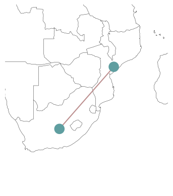
Since we have provided x and y coordinates for our buses, n.plot() will try to plot the network on a map by default. Of course, there’s an option to deactivate this behaviour:
n.plot(geomap=False)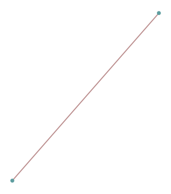
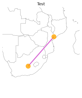
The n.plot() function has a variety of styling arguments to tweak the appearance of the buses, the lines and the map in the background:
n.plot(
    margin=1,
    bus_sizes=1,
    bus_colors="orange",
    bus_alpha=0.8,
    line_colors="orchid",
    line_widths=3,
    title="Test",
)
We can use the bus_sizes argument of n.plot() to display the regional distribution of load. First, we calculate the total load per bus:
s = n.loads.groupby("bus").p_set.sum() / 1e4
s
bus
MZ 0.065
SA 4.200
Name: p_set, dtype: float64The resulting pandas.Series we can pass to n.plot(bus_sizes=...):
n.plot(margin=1, bus_sizes=s)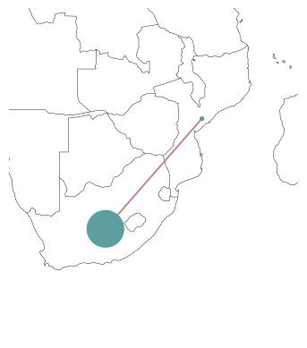
The important point here is, that s needs to have entries for all buses, i.e. its index needs to match n.buses.index.
The bus_sizes argument of n.plot() can be even more powerful. It can produce pie charts, e.g. for the mix of electricity generation at each bus.
The dispatch of each generator, we can find at:
n.generators_t.p.loc["now"]name
MZ hydro 1150.0
SA coal 35000.0
SA wind 3000.0
SA gas 1500.0
SA oil 2000.0
Name: now, dtype: float64If we group this by the bus and carrier...
n.generators.carriername
MZ hydro hydro
SA coal coal
SA wind wind
SA gas gas
SA oil oil
Name: carrier, dtype: object... we get a multi-indexed pandas.Series ...
s = n.generators_t.p.loc["now"].groupby([n.generators.bus, n.generators.carrier]).sum()
s
bus carrier
MZ hydro 1150.0
SA coal 35000.0
gas 1500.0
oil 2000.0
wind 3000.0
Name: now, dtype: float64... which we can pass to n.plot(bus_sizes=...):
n.plot(margin=1, bus_sizes=s / 3000)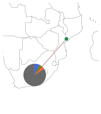
How does this magic work? The plotting function will look up the colors specified in n.carriers for each carrier and match it with the second index-level of s.
Besides the static plots with n.plot(), PyPSA also has an interactive plotting function n.explore(), which renders the network on a zoomable map. We will see more of it in the SciGRID example below, but it already works for our small two-country network:
n.explore()Modifying networks
Modifying data of components in an existing PyPSA network is as easy as modifying the entries of a pandas.DataFrame. For instance, if we want to reduce the cross-border transmission capacity between South Africa and Mozambique, we’d run:
n.lines.loc["SA-MZ", "s_nom"] = 100
n.linesn.optimize(solver_name="highs", log_to_console=False)INFO:linopy.model: Solve problem using Highs solver
INFO:linopy.model:Solver options:
 - log_to_console: False
INFO:linopy.io: Writing time: 0.03s
INFO:linopy.constants: Optimization successful:
Status: ok
Termination condition: optimal
Solution: 6 primals, 14 duals
Objective: 1.45e+06
Solver: highs
Runtime: 0.00s
MIP gap: inf
Dual bound: 0.00e+00
Solver model: available
Solver message: Optimal
INFO:pypsa.optimization.optimize:The shadow-prices of the constraints Generator-fix-p-lower, Generator-fix-p-upper, Line-fix-s-lower, Line-fix-s-upper were not assigned to the network.
('ok', 'optimal')You can see that the production of the hydro power plant was reduced and that of the gas power plant increased owing to the reduced transmission capacity.
n.generators_t.pGlobal constraints for emission limits
In the example above, we happen to have some spare gas capacity with lower carbon intensity than the coal and oil generators. We could use this to lower the emissions of the system, but it will be more expensive. We can implement the limit of carbon dioxide emissions as a constraint.
This is achieved in PyPSA through Global Constraints which add constraints that apply to many components at once.
But first, we need to calculate the current level of emissions to set a sensible limit.
We can compute the emissions per generator (in tonnes of CO) in the following way.
where is the specific emissions (tonnes/MWh thermal) and is the conversion efficiency (MWh electric / MWh thermal) of the generator with dispatch (MWh electric):
e = (
    n.generators_t.p
    / n.generators.efficiency
    * n.generators.carrier.map(n.carriers.co2_emissions)
)
eSummed up, we get total emissions in tonnes:
e.sum().sum()np.float64(38201.49276011344)So, let’s say we want to reduce emissions by 10%:
n.add(
    "GlobalConstraint",
    "emission_limit",
    carrier_attribute="co2_emissions",
    sense="<=",
    constant=e.sum().sum() * 0.9,
)
Let’s check how the new global constraint looks like in the optimisation problem:
n.optimize.create_model()
n.model.constraints["GlobalConstraint-emission_limit"]
Constraint `GlobalConstraint-emission_limit`
--------------------------------------------
+1.03 Generator-p[now, SA coal] + 0.3448 Generator-p[now, SA gas] + 0.7429 Generator-p[now, SA oil] ≤ 34381.3434841021n.optimize(solver_name="highs", log_to_console=False)INFO:linopy.model: Solve problem using Highs solver
INFO:linopy.model:Solver options:
 - log_to_console: False
INFO:linopy.io: Writing time: 0.03s
INFO:linopy.constants: Optimization successful:
Status: ok
Termination condition: optimal
Solution: 6 primals, 15 duals
Objective: 2.21e+06
Solver: highs
Runtime: 0.00s
MIP gap: inf
Dual bound: 0.00e+00
Solver model: available
Solver message: Optimal
INFO:pypsa.optimization.optimize:The shadow-prices of the constraints Generator-fix-p-lower, Generator-fix-p-upper, Line-fix-s-lower, Line-fix-s-upper were not assigned to the network.
('ok', 'optimal')n.generators_t.pn.generators_t.p / n.generators.p_nomThe shadow price of the emission limit tells us by how much the system cost would decrease if we allowed one more tonne of CO:
n.global_constraints.muname
emission_limit -392.771084
Name: mu, dtype: float64Can we lower emissions even further? Say by another 5% points?
n.global_constraints.loc["emission_limit", "constant"] = e.sum().sum() * 0.85n.optimize(solver_name="highs", log_to_console=False)INFO:linopy.model: Solve problem using Highs solver
INFO:linopy.model:Solver options:
 - log_to_console: False
INFO:linopy.io: Writing time: 0.03s
WARNING:linopy.constants:Optimization potentially failed:
Status: warning
Termination condition: infeasible
Solution: 0 primals, 0 duals
Objective: nan
Solver: highs
Runtime: 0.00s
MIP gap: inf
Dual bound: 0.00e+00
Solver model: available
Solver message: Infeasible
('warning', 'infeasible')No! Without any additional capacities, we have exhausted our options to reduce emissions in that hour. The solver tells us that the problem is infeasible, i.e. there is no solution that satisfies all constraints. Better revert this change:
n.global_constraints.loc["emission_limit", "constant"] = e.sum().sum() * 0.9Data import and export
You may find yourself in a need to store PyPSA networks for later use. Or, maybe you want to import the genius PyPSA example that someone else uploaded to the web to explore.
Among other file formats, PyPSA networks can be stored as netCDF (.nc) files, as folders of CSV files, or as Excel (.xlsx) files.
netCDFfiles have the advantage that they take up less space thanCSVfiles and are faster to load.CSVandExcelmight be easier to inspect by hand.
The approach is similar for all formats:
n.export_to_netcdf("tmp.nc");INFO:pypsa.network.io:Exported network 'Unnamed Network' saved to 'tmp.nc contains: sub_networks, generators, loads, buses, carriers, lines, global_constraints
n_nc = pypsa.Network("tmp.nc")
n_nc
INFO:pypsa.network.io:New version 1.3.0 available! (Current: 1.2.4)
INFO:pypsa.network.io:Imported network 'Unnamed Network' has buses, carriers, generators, global_constraints, lines, loads, sub_networks
PyPSA Network 'Unnamed Network'
-------------------------------
Components:
 - Bus: 2
 - Carrier: 6
 - Generator: 5
 - GlobalConstraint: 1
 - Line: 1
 - Load: 2
 - SubNetwork: 1
Snapshots: 1
Example grid model with time resolution
Dispatch problem with German SciGRID network
SciGRID is a project that provides an open reference model of the European transmission network. The network comprises time series for loads and the availability of renewable generation at an hourly resolution for January 1, 2011 as well as approximate generation capacities in 2014. This dataset is a little out of date and only intended to demonstrate the capabilities of PyPSA.
We load it as a second network n2, so that our two-country network n stays available for the exercises at the end:
n2 = pypsa.examples.scigrid_de()INFO:pypsa.examples:Downloading https://data.pypsa.org/networks/examples/v1.2.4/scigrid_de.nc to /home/runner/.cache/pypsa/examples/v1.2.4/scigrid_de.nc
INFO:pypsa.network.io:New version 1.3.0 available! (Current: 1.2.4)
INFO:pypsa.network.io:Imported network 'SciGrid-DE' has buses, carriers, generators, lines, loads, storage_units, transformers
There are some infeasibilities without allowing extension. Moreover, to approximate so-called security, we don’t allow any line to be loaded above 70% of their thermal rating. security is a constraint that states that no single transmission line may be overloaded by the failure of another transmission line (e.g. through a tripped connection).
n2.lines.s_max_pu = 0.7
n2.lines.loc[["316", "527", "602"], "s_nom"] = 1715
Because this network includes time-varying data, now is the time to look at another attribute of n: n.snapshots. Snapshots is the PyPSA terminology for time steps. In most cases, they represent a particular hour. They can be a pandas.DatetimeIndex or any other list-like attributes.
n2.snapshots[:4]DatetimeIndex(['2011-01-01 00:00:00', '2011-01-01 01:00:00',
'2011-01-01 02:00:00', '2011-01-01 03:00:00'],
dtype='datetime64[ns]', name='snapshot', freq=None)This index will match with any time-varying attributes of components:
n2.loads_t.p_set.iloc[:3, :3]We can use simple pandas syntax, to create an overview of the load time series...
n2.loads_t.p_set.sum(axis=1).plot(ylim=[0, 60e3], ylabel="MW")<Axes: xlabel='snapshot', ylabel='MW'>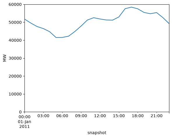
... and the capacity factor time series of the renewable generators:
n2.generators_t.p_max_pu.T.groupby(n2.generators.carrier).mean().T.plot(ylabel="p.u.")<Axes: xlabel='snapshot', ylabel='p.u.'>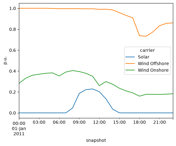
We can also inspect the total power plant capacities per technology:
n2.generators.groupby("carrier").p_nom.sum().div(1e3).sort_values().plot.barh(
    xlabel="GW"
)
<Axes: xlabel='GW', ylabel='carrier'>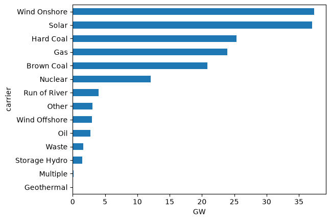
Interactive network plotting
The network inputs and outputs can also be visualised on a map. The n.plot() function we already know uses matplotlib to create static plots, while n.explore() creates interactive plots based on pydeck. In the following, we will focus on the interactive plotting with n.explore().
The n.explore() function has a variety of styling arguments to tweak the appearance of the buses, the lines and the map in the background. For example, we can size the buses according to their load:
load = n2.loads_t.p_set.sum(axis=0).groupby(n2.loads.bus).sum()
load.head(3)
bus
1 5417.262030
100_220kV 465.763014
101 1382.220699
dtype: float64n2.explore(bus_size=load / 20)The bus_size argument of n.explore() can be even more powerful. It can show the nodal composition of power plant capacities as pie charts by grouping data by the bus and carrier attributes of the generators:
capacities = n2.generators.groupby(["bus", "carrier"]).p_nom.sum()
capacities.head(3)
bus carrier
1 Gas 121.000000
Hard Coal 272.000000
Solar 79.674256
Name: p_nom, dtype: float64... for which we need to assign some colors to the technologies first:
colors = {
    "Gas": "tomato",
    "Hard Coal": "dimgrey",
    "Run of River": "turquoise",
    "Waste": "olive",
    "Brown Coal": "peru",
    "Oil": "black",
    "Storage Hydro": "teal",
    "Other": "whitesmoke",
    "Multiple": "whitesmoke",
    "Nuclear": "deeppink",
    "Geothermal": "darkorange",
    "Wind Offshore": "lightskyblue",
    "Wind Onshore": "royalblue",
    "Solar": "gold",
    "Pumped Hydro": "lightseagreen",
    "AC": "crimson",
}
n2.add("Carrier", colors.keys(), color=colors.values(), overwrite=True)
n2.explore(bus_size=capacities / 3)So let’s solve the electricity market simulation for January 1, 2011. It’ll take a short moment.
n2.optimize(solver_name="highs", log_to_console=False)WARNING:pypsa.consistency:The following transformers have zero r, which could break the linear load flow:
Index(['2', '5', '10', '12', '13', '15', '18', '20', '22', '24', '26', '30',
'32', '37', '42', '46', '52', '56', '61', '68', '69', '74', '78', '86',
'87', '94', '95', '96', '99', '100', '104', '105', '106', '107', '117',
'120', '123', '124', '125', '128', '129', '138', '143', '156', '157',
'159', '160', '165', '184', '191', '195', '201', '220', '231', '232',
'233', '236', '247', '248', '250', '251', '252', '261', '263', '264',
'267', '272', '279', '281', '282', '292', '303', '307', '308', '312',
'315', '317', '322', '332', '334', '336', '338', '351', '353', '360',
'362', '382', '384', '385', '391', '403', '404', '413', '421', '450',
'458'],
dtype='object', name='name')
INFO:linopy.model: Solve problem using Highs solver
INFO:linopy.model:Solver options:
 - log_to_console: False
INFO:linopy.io:Writing objective.
Writing constraints.: 0%| | 0/15 [00:00<?, ?it/s]Writing constraints.: 87%|████████▋ | 13/15 [00:00<00:00, 109.69it/s]Writing constraints.: 100%|██████████| 15/15 [00:00<00:00, 82.10it/s]
Writing continuous variables.: 0%| | 0/6 [00:00<?, ?it/s]Writing continuous variables.: 100%|██████████| 6/6 [00:00<00:00, 275.53it/s]
INFO:linopy.io: Writing time: 0.22s
INFO:linopy.constants: Optimization successful:
Status: ok
Termination condition: optimal
Solution: 59640 primals, 142968 duals
Objective: 9.20e+06
Solver: highs
Runtime: 6.41s
MIP gap: inf
Dual bound: 0.00e+00
Solver model: available
Solver message: Optimal
INFO:pypsa.optimization.optimize:The shadow-prices of the constraints Generator-fix-p-lower, Generator-fix-p-upper, Line-fix-s-lower, Line-fix-s-upper, Transformer-fix-s-lower, Transformer-fix-s-upper, StorageUnit-fix-p_dispatch-lower, StorageUnit-fix-p_dispatch-upper, StorageUnit-fix-p_store-lower, StorageUnit-fix-p_store-upper, StorageUnit-fix-state_of_charge-lower, StorageUnit-fix-state_of_charge-upper, Kirchhoff-Voltage-Law, StorageUnit-energy_balance were not assigned to the network.
('ok', 'optimal')Now, we can also plot model outputs, like the calculated power flows on the network map using the line_flow argument of n.explore():
line_loading = (
    n2.lines_t.p0.iloc[0].abs() / n2.lines.s_nom / n2.lines.s_max_pu * 100
)  # %
n2.explore(
bus_size=1e1,
line_color=line_loading.abs(),
line_flow=n2.lines_t.p0.iloc[0] / 100,
line_cmap="plasma",
line_width=n2.lines.s_nom / 1000,
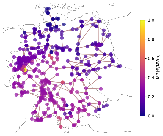
)Static plots remain useful for reports and publications. For instance, we can plot the average locational marginal prices (LMPs) with n.plot():
fig = plt.figure(figsize=(7, 7))
ax = plt.axes(projection=ccrs.EqualEarth())

n2.plot(
    ax=ax,
    bus_colors=n2.buses_t.marginal_price.mean(),
    bus_cmap="plasma",
    bus_alpha=0.7,
)

plt.colorbar(
    plt.cm.ScalarMappable(cmap="plasma"),
    ax=ax,
    label="LMP [€/MWh]",
    shrink=0.6,
)
Statistics
The PyPSA n.statistics module provides a variety of pre-defined tables and plots to analyse optimisation results at different aggregation levels. For instance, the energy balance, the operational costs (OPEX), curtailment, prices and market value. We will use this module in more detail later in this workshop.
For example, we can plot the hourly dispatch grouped by carrier with a single line of code:
n2.statistics.energy_balance.iplot()Or look at the energy balance as a table (in GWh):
n2.statistics.energy_balance().div(1e3).round(1).sort_values()component carrier bus_carrier
Load - AC -1210.0
StorageUnit Pumped Hydro AC -2.7
Generator Geothermal AC 0.2
Other AC 3.7
Gas AC 5.5
Storage Hydro AC 25.3
Wind Offshore AC 31.0
Waste AC 33.5
Solar AC 46.2
Run of River AC 83.0
Nuclear AC 176.6
Hard Coal AC 185.4
Brown Coal AC 215.2
Wind Onshore AC 407.2
dtype: float64Or the operational costs (OPEX) per technology:
n2.statistics.opex().round(1).sort_values(ascending=False)component carrier
Generator Hard Coal 4634772.9
Brown Coal 2151669.5
Nuclear 1412597.8
Gas 276634.6
Run of River 248924.6
Waste 200916.7
Other 117165.7
StorageUnit Pumped Hydro 75904.9
Generator Storage Hydro 75896.4
Geothermal 4804.8
dtype: float64There is much more to explore in PyPSA. If you are hooked, have a look at the documentation and the examples section.
Exercises
Modify some of the input data of the South Africa & Mozambique network n, first removing the emission limit global constraint:
n.remove("GlobalConstraint", "emission_limit")Task 1: Model an outage of the transmission line by removing it. How does the model compensate for the lack of transmission?
n.model.solver_model = None
n_t1 = n.copy()

n_t1.remove("Line", "SA-MZ")
n_t1.optimize(solver_name="highs", log_to_console=False)
INFO:linopy.model: Solve problem using Highs solver
INFO:linopy.model:Solver options:
 - log_to_console: False
INFO:linopy.io: Writing time: 0.02s
INFO:linopy.constants: Optimization successful:
Status: ok
Termination condition: optimal
Solution: 5 primals, 12 duals
Objective: 1.47e+06
Solver: highs
Runtime: 0.00s
MIP gap: inf
Dual bound: 0.00e+00
Solver model: available
Solver message: Optimal
INFO:pypsa.optimization.optimize:The shadow-prices of the constraints Generator-fix-p-lower, Generator-fix-p-upper were not assigned to the network.
('ok', 'optimal')n_t1.statistics.energy_balance().astype(int).sort_values()component carrier bus_carrier
Load Electricity Electricity -42650
Generator Hydro Electricity 650
Oil Electricity 2000
Gas Electricity 2000
Onshore Wind Electricity 3000
Coal Electricity 35000
dtype: int64Task 2: Double the wind capacity. How is the electricity price in South Africa affected? What generator is price-setting?
n.model.solver_model = None
n_t2 = n.copy()

n_t2.generators.loc["SA wind", "p_nom"] *= 2
n_t2.optimize(solver_name="highs", log_to_console=False)
INFO:linopy.model: Solve problem using Highs solver
INFO:linopy.model:Solver options:
 - log_to_console: False
INFO:linopy.io: Writing time: 0.03s
INFO:linopy.constants: Optimization successful:
Status: ok
Termination condition: optimal
Solution: 6 primals, 14 duals
Objective: 9.72e+05
Solver: highs
Runtime: 0.00s
MIP gap: inf
Dual bound: 0.00e+00
Solver model: available
Solver message: Optimal
INFO:pypsa.optimization.optimize:The shadow-prices of the constraints Generator-fix-p-lower, Generator-fix-p-upper, Line-fix-s-lower, Line-fix-s-upper were not assigned to the network.
('ok', 'optimal')price = n_t2.buses_t.marginal_price
pricen_t2.generators.loc[
n.generators.marginal_cost.round(2) == price.at["now", "SA"].round(2)
].index[0]'SA oil'Task 3: South Africa brings a new 1000 MW nuclear power plant into operation with an estimated marginal electricity generation cost of 20 €/MWh. Will that affect the electricity price?
n.model.solver_model = None
n_t3 = n.copy()

n_t3.add(
    "Generator",
    "SA nuclear",
    bus="SA",
    carrier="nuclear",
    p_nom=1000,
    marginal_cost=20,
)
n_t3.optimize(solver_name="highs", log_to_console=False)
WARNING:pypsa.consistency:The following generators have carriers which are not defined. Run n.sanitize() to add them. Components with undefined carriers:
Index(['SA nuclear'], dtype='object', name='name')
INFO:linopy.model: Solve problem using Highs solver
INFO:linopy.model:Solver options:
 - log_to_console: False
INFO:linopy.io: Writing time: 0.02s
INFO:linopy.constants: Optimization successful:
Status: ok
Termination condition: optimal
Solution: 7 primals, 16 duals
Objective: 1.30e+06
Solver: highs
Runtime: 0.00s
MIP gap: inf
Dual bound: 0.00e+00
Solver model: available
Solver message: Optimal
INFO:pypsa.optimization.optimize:The shadow-prices of the constraints Generator-fix-p-lower, Generator-fix-p-upper, Line-fix-s-lower, Line-fix-s-upper were not assigned to the network.
('ok', 'optimal')n_t3.buses_t.marginal_price